Why Do We Perform Statistical Analysis? (Advanced)
Our advanced articles describe how our features/systems work in detail and will sometimes require knowledge of certain scientific or technical terms.
A/B testing is a data driven way of optimizing a game. Thus, an experiment starts with collecting data from each variant. Each variant has a latent property that we want to compare. For example, to test binary goal metrics, we assume that the user sets of each variants have a latent true conversion rate. To test playtime per user data, we assume that there is a latent session length distribution that generates our measurements.
For example, consider the following binary A/B test:
| Variant | True Conversion Rate | Number of users | Converted users – measurements |
|---|---|---|---|
| “Control” | 0.11 | 10000 | 1110 |
| “A” | 0.13 | 10000 | 1290 |
As we see in the table above, data collection is probabilistic in nature: for a true conversion rate of 0.11, we may not always end up with 11% of converted users. This is due to the fact that our sample is a subset of the overall population. In our case, that would be every single user that would ever play the game; our sample would be the users that happen to be acquired for the experiment. For this reason, inferring latent factors from measurements is not a one-to-one relationship.
For example, let us try to infer the true conversion rate of the control variant in the table above. We may argue that it is highly unlikely that a true conversion rate of 0.01 generated such results. Similarly, it is quite apparent that the true conversion rate is most probably not 0.5. The likely conversion rates are centered around the value 0.111. This relationship is usually represented in models by probability densities.
To determine the conversion rate densities given the measured data, we may perform Bayesian inference. The outcome of bayesian inference may be the following:
On the vertical axis, you can see the probability density of a conversion rate value given the measurements of the variant. To calculate the probability of a variant being the winner, we first sample conversion rate values from these probability densities. After that, we compare these samples one-to-one, hence deriving the probability.
You can see an example of this in the following table:
| Sample | Index | Conversion rate “Control” | Conversion rate “A” | Winner |
|---|---|---|---|---|
| 315 | 1 | 0.11472557 | 0.12875037 | “A” |
| 256 | 2 | 0.10708776 | 0.12445933 | “A” |
| 127 | 3 | 0.11878974 | 0.12853538 | “A” |
| 538 | 4 | 0.11921174 | 0.11852222 | “Control” |
| … | ... | … | … | … |
| N | N | 0.1101358 | 0.13813024 | “A” |
After collecting a sufficient number of samples, one may realize that – what we ended up with using simple common sense arguments is mathematically justified – the probability that version “A” performs better than control is 0.998.
For some other experiment, we may end up with the following probability distributions:
Here, we can see that there is no significant difference between the variants.
The analysis outlined above is applicable for more than one variant. Imagine the following conversion data was measured in an A/B testing experiment with 4 variants:
| Variant | Number of users | Converted Users |
|---|---|---|
| “Control” | 2000 | 110 |
| “A” | 2001 | 100 |
| “B” | 1999 | 105 |
| “C” | 2000 | 104 |
After performing Bayesian inference, the probability densities of the conversion rates have the following form:
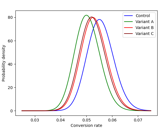
Among the probability densities above, we cannot find one, that may be distinctively greater than all the others. In fact, if we sample a sufficiently high number of conversion rate values from the probability distributions of the variants, and compare them, we will see that none of the variants’ winning percentages are dominant above the others, indicating that the measurements are not significantly different:
| Variant | Winning Percentage |
|---|---|
| “Control” | 44.5% |
| “A” | 11.3% |
| “B” | 24.1% |
| “C” | 20.1% |
And also, we could compute the relations of individual variants,
| Variant | Percentage |
|---|---|
| P ( “Control” performs better than “A” ) | 76.5 % |
| P ( “Control” performs better than “B” ) | 63.0% |
| P( “Control” performs better than “C” ) | 66.5% |
| P ( “A” performs better than “B” ) | 34.9% |
| P ( “A” performs better than “C” ) | 38.4% |
| P ( “B” performs better than “C” ) | 53.2% |
Different variants will naturally produce different measurement results. For example, let’s say that an experiment starts running, and after two days, the collected data shows that the mean playtime of a variant has increased by 10%. This does not necessarily mean that this variant is significantly better than the others. It may be that the number of collected samples is low, and there is an outlier – maybe a test device – that contributed to the variant. So, in order to draw reliable conclusions from these differences, A/B testing is concluded by thorough statistical analysis, to assess whether the measurement differences simply occurred by chance, or if there is a statistically significant difference between the variants.
For example, imagine we are trying to find the best difficulty level of a game in order to keep as many players as possible after a week. Assume the control variant corresponds to a medium level of difficulty, and variant “A” is slightly easier. Consider the following day 7 retention measurements:
| Variant | Number of users | Returning users |
|---|---|---|
| “Control” | 2000 | 110 |
| “A” | 2001 | 112 |
The measurements above are very close, it is highly probable that there is no significant difference between the conversion of the two variants. The following measurements however differ to a greater extent.
| Variant | Number of users | Returning users |
|---|---|---|
| “Control” | 2000 | 110 |
| “A” | 2001 | 220 |
These measurements suggest that variant “A” is significantly more likely to attract users, than the control variant. In the second example, it seems evident that the probability of users returning after 7 days is significantly higher than in the first example. With A/B testing, game developers can perform similar common-sense reasoning in a data-driven, mathematically rigorous manner.